Crossover analysis

import numpy as np
import matplotlib.pyplot as plt
import geoviews.feature as gf
import cartopy.crs as ccrs
from concurrent.futures import ThreadPoolExecutor
from tqdm import tqdm

import xopr

import holoviews as hv
import hvplot.pandas
hvplot.extension('bokeh')

# Useful background features for maps
background_map = gf.ocean.opts(projection=ccrs.SouthPolarStereo(true_scale_latitude=-71), scale='50m') * gf.coastline.opts(projection=ccrs.SouthPolarStereo(true_scale_latitude=-71), scale='50m')

# Establish an OPR session
# Setting a cache directory speeds up subsequent requests when running locally.
opr = xopr.OPRConnection(cache_dir="radar_cache")

regions_df = xopr.geometry.get_antarctic_regions(merge_regions=False).to_crs('EPSG:3031')
regions_df.hvplot(frame_width=600, aspect='equal', hover_cols=['NAME'], c='TYPE')

region = xopr.geometry.get_antarctic_regions(name="David", merge_regions=True, simplify_tolerance=100, type='GR')
region_projected = xopr.geometry.project_geojson(region, source_crs='EPSG:4326', target_crs="EPSG:3031")

region_hv = hv.Polygons([region_projected]).opts(
    color='green',
    line_color='black',
    fill_alpha=0.5)

(background_map * region_hv).opts(aspect='equal')

stac_items_df = opr.query_frames(geometry=region) # Can also add a date range: date_range="2020-01-01T00:00:00Z/2024-01-01T00:00:00Z"
stac_items_df = stac_items_df.to_crs('EPSG:3031')

print(f"Found {len(stac_items_df)} frames across {stac_items_df['collection'].nunique()} collections:")
stac_items_df.groupby('collection').size()

flight_lines = stac_items_df.hvplot(by='collection')
(background_map * region_hv * flight_lines).opts(frame_width=500, aspect='equal', active_tools=['pan', 'wheel_zoom'])

intersections = xopr.find_intersections(stac_items_df, calculate_crossing_angles=True)

intersections = intersections[intersections['crossing_angle'] > 2] # Filter out nearly coincident crossings

print(f"Found {len(intersections)} crossover points between flight lines.")
(background_map * region_hv * flight_lines * intersections.hvplot(label='Intersection Points', c='crossing_angle')).opts(frame_width=500, aspect='equal', active_tools=['pan', 'wheel_zoom'])

intersections.head()

def nearest_trace(ds, x, y):
    """Return the index of the trace in a projected dataset closest to (x, y)."""
    return np.argmin(((ds['x'] - x)**2 + (ds['y'] - y)**2).data)

def get_bed_wgs84(item_id):
    """Load layers for a frame and return the bed pick with WGS84 elevation, projected to EPSG:3031."""
    layers = opr.get_layers(stac_items_df.loc[item_id].to_dict())
    if layers is None or 'standard:bottom' not in layers:
        return None
    bed = xopr.layer_twtt_to_range(layers['standard:bottom'], layers['standard:surface'], vertical_coordinate='wgs84')
    return xopr.geometry.project_dataset(bed.rename({'lat': 'Latitude', 'lon': 'Longitude'}), 'EPSG:3031')

# Fetch layers for each unique frame in parallel (each frame appears in many crossovers)
frame_ids = np.unique(intersections[['id_1', 'id_2']].to_numpy())
with ThreadPoolExecutor(max_workers=8) as pool:
    beds = dict(zip(frame_ids, tqdm(pool.map(get_bed_wgs84, frame_ids), total=len(frame_ids))))

def crossover_error(row):
    """Bed elevation from each frame at the crossover point, and the distance between the two picks."""
    bed_1, bed_2 = beds[row['id_1']], beds[row['id_2']]
    if bed_1 is None or bed_2 is None:
        return np.nan, np.nan, np.nan
    x, y = row.intersection_geometry.coords[0]
    i, j = nearest_trace(bed_1, x, y), nearest_trace(bed_2, x, y)
    dist = np.sqrt((bed_1['x'][i] - bed_2['x'][j])**2 + (bed_1['y'][i] - bed_2['y'][j])**2)
    return bed_1['wgs84'][i].item(), bed_2['wgs84'][j].item(), dist.item()

intersections[['wgs84_1', 'wgs84_2', 'layer_pt_distance']] = intersections.apply(crossover_error, axis=1, result_type='expand')

intersections['elev_diff'] = np.abs(intersections['wgs84_1'] - intersections['wgs84_2'])
# Set elev_diff to NaN where layer_pt_distance is large
intersections.loc[intersections['layer_pt_distance'] > 100, 'elev_diff'] = np.nan

intersections_success = intersections.dropna(subset=['wgs84_1', 'wgs84_2', 'elev_diff', 'layer_pt_distance']).reset_index(drop=True)

# Report how many intersections had valid layer data
n_total = len(intersections)
n_success = len(intersections_success)
print(f"Layer data available for {n_success}/{n_total} intersections ({100*n_success/n_total:.0f}%)")

if len(intersections_success) == 0:
    raise ValueError("No intersections with valid layer data found. Try expanding the date range or choosing a different region.")

intersections_success['intersection_geometry_x'] = intersections_success['intersection_geometry'].apply(lambda geom: geom.x)
intersections_success = intersections_success.sort_values(by='intersection_geometry_x', ascending=False).reset_index(drop=True)
intersections_success['idx'] = intersections_success.index
hover_tooltips = [
    ("Index", "@idx"),
    ("Collection 1", "@collection_1"),
    ("Collection 2", "@collection_2"),
    ("Difference", "@elev_diff{0.00} m"),
]

vlim = intersections_success['elev_diff'].abs().quantile(0.99)

hv_int = intersections_success.hvplot(color='elev_diff', hover_cols=['idx', 'collection_1', 'collection_2', 'elev_diff'], hover_tooltips=hover_tooltips, clim=(0, vlim))
#hv_int = hv_int.opts(scalebar=True) # Can enable if you want - requires hvplot >= 0.12.0
(background_map * region_hv * flight_lines * hv_int).opts(frame_width=600, aspect='equal', active_tools=['pan', 'wheel_zoom'])

import xarray as xr
import earthaccess

def earthdata_login():
    """Try non-interactive Earthdata login strategies; return True if one succeeds."""
    for strategy in ['environment', 'netrc']:
        try:
            if earthaccess.login(strategy=strategy).authenticated:
                return True
        except Exception:
            pass
    return False

# Fetch BedMachine Antarctica v4 from NSIDC and subset to our region.
# If no Earthdata credentials are stored, bed_bm stays None and the comparison cells are skipped.
bed_bm = None
if earthdata_login():
    bm_files = earthaccess.open(earthaccess.search_data(short_name='NSIDC-0756', version='4', count=1))
    bm = xr.open_dataset(bm_files[0])
    xmin, ymin, xmax, ymax = intersections_success.total_bounds
    pad = 15e3
    bm = bm.sel(x=slice(xmin - pad, xmax + pad), y=slice(ymax + pad, ymin - pad))  # y is descending
    bed_bm = bm['bed'] + bm['geoid']  # geoid-referenced -> WGS84 ellipsoidal, to match the radar picks
else:
    print("No Earthdata credentials found -- skipping the BedMachine comparison.")

# Interpolate BedMachine at each crossover and difference against the mean of the two radar picks
if bed_bm is not None:
    pts = intersections_success.intersection_geometry
    intersections_success['bedmachine'] = bed_bm.interp(x=xr.DataArray(pts.x), y=xr.DataArray(pts.y)).values
    intersections_success['bedmachine_diff'] = \
        intersections_success[['wgs84_1', 'wgs84_2']].mean(axis=1) - intersections_success['bedmachine']

    print(f"Radar minus BedMachine: mean {intersections_success['bedmachine_diff'].mean():.1f} m, "
          f"median {intersections_success['bedmachine_diff'].median():.1f} m")

    vlim_bm = intersections_success['bedmachine_diff'].abs().quantile(0.9)
    hv_bm = intersections_success.hvplot(color='bedmachine_diff', hover_cols=['idx', 'elev_diff', 'bedmachine_diff'],
                                         clim=(-vlim_bm, vlim_bm), cmap='RdBu_r', clabel='Radar - BedMachine (m)')
    display((background_map * region_hv * flight_lines * hv_bm).opts(frame_width=600, aspect='equal', active_tools=['pan', 'wheel_zoom']))

# Select an index to investigate - pick one from the map above, or use a default
# We default to the intersection with the largest elevation difference
print(f"Valid index range: 0 to {len(intersections_success)-1}")
selected_idx = intersections_success['elev_diff'].argmax()
print(f"Selected index: {selected_idx}")

# Load both frames, interpolate to a WGS84 elevation grid, and find the trace nearest the crossover
intersect = intersections_success.loc[selected_idx]
x_int, y_int = intersect.intersection_geometry.coords[0]

frames, cross_idxs = [], []
for item_id in [intersect['id_1'], intersect['id_2']]:
    frame = opr.load_frame(stac_items_df.loc[item_id].to_dict())
    frame = xopr.radar_util.add_along_track(frame)
    frame = xopr.radar_util.interpolate_to_vertical_grid(frame, vertical_coordinate='wgs84')
    frame = xopr.geometry.project_dataset(frame, 'EPSG:3031')
    frames.append(frame)
    cross_idxs.append(nearest_trace(frame, x_int, y_int))

print(f"Frame 1: {intersect['id_1']} from {intersect['collection_1']}")
print(f"Frame 2: {intersect['id_2']} from {intersect['collection_2']}")
print(f"Intersection at trace {cross_idxs[0]} (frame 1) and {cross_idxs[1]} (frame 2)")
print(f"Bed elevation difference: {intersect['elev_diff']:.2f} m")

def load_layers_wgs84(frame):
    """Load layers for a frame, drop empty ones, and add along-track distance and WGS84 elevation."""
    layers = {name: l for name, l in opr.get_layers(frame).items() if l.sizes.get('slow_time', 0) > 0}
    surface = layers['standard:surface']
    return {name: xopr.layer_twtt_to_range(xopr.radar_util.add_along_track(l), surface, vertical_coordinate='wgs84')
            for name, l in layers.items()}

frame_layers = [load_layers_wgs84(f) for f in frames]

# Sample BedMachine along each track and add it as an extra "layer" so it gets plotted too
if bed_bm is not None:
    for f, layers in zip(frames, frame_layers):
        layers['BedMachine'] = xr.Dataset({'wgs84': bed_bm.interp(x=f['x'], y=f['y'])})

def plot_radargram(frame, layers, idx, ax, title, zoom=None):
    """Plot a radargram in WGS84 elevation coordinates with layer picks and a crossover marker.

    zoom, if given, is a (n_traces, elev_window_m) tuple to zoom in around the crossover."""
    pwr = 10*np.log10(np.abs(frame.Data))
    vmin, vmax = np.percentile(pwr, [30, 97])
    pwr.plot.imshow(x='along_track', y='wgs84', cmap='gray', ax=ax, vmin=vmin, vmax=vmax)
    ax.axvline(frame.along_track[idx], color='red', linestyle='--', linewidth=2, label='Crossover')
    for name, layer in layers.items():
        layer['wgs84'].plot(ax=ax, x='along_track', linewidth=1, linestyle=':', label=name)
    if zoom is not None:
        n_traces, elev_window = zoom
        lo, hi = max(0, idx - n_traces), min(frame.sizes['slow_time'] - 1, idx + n_traces)
        ax.set_xlim(frame.along_track[lo], frame.along_track[hi])
        bed = layers['standard:bottom']['wgs84'].sel(slow_time=frame.slow_time[idx], method='nearest').item()
        ax.set_ylim(bed - elev_window/2, bed + elev_window/2)
    ax.set_title(title)
    ax.set_ylabel('Elevation (m)')
    ax.legend()

fig, axes = plt.subplots(2, 1, figsize=(15, 8))
for k, ax in enumerate(axes):
    plot_radargram(frames[k], frame_layers[k], cross_idxs[k], ax,
                   f"{intersect[f'collection_{k+1}']} - {intersect[f'id_{k+1}']} (Elevation view)")
axes[1].set_xlabel('Along track distance (m)')
plt.suptitle(f"Radargrams in elevation coordinates - Bed elev diff: {intersect['elev_diff']:.2f} m", fontsize=14)
plt.tight_layout()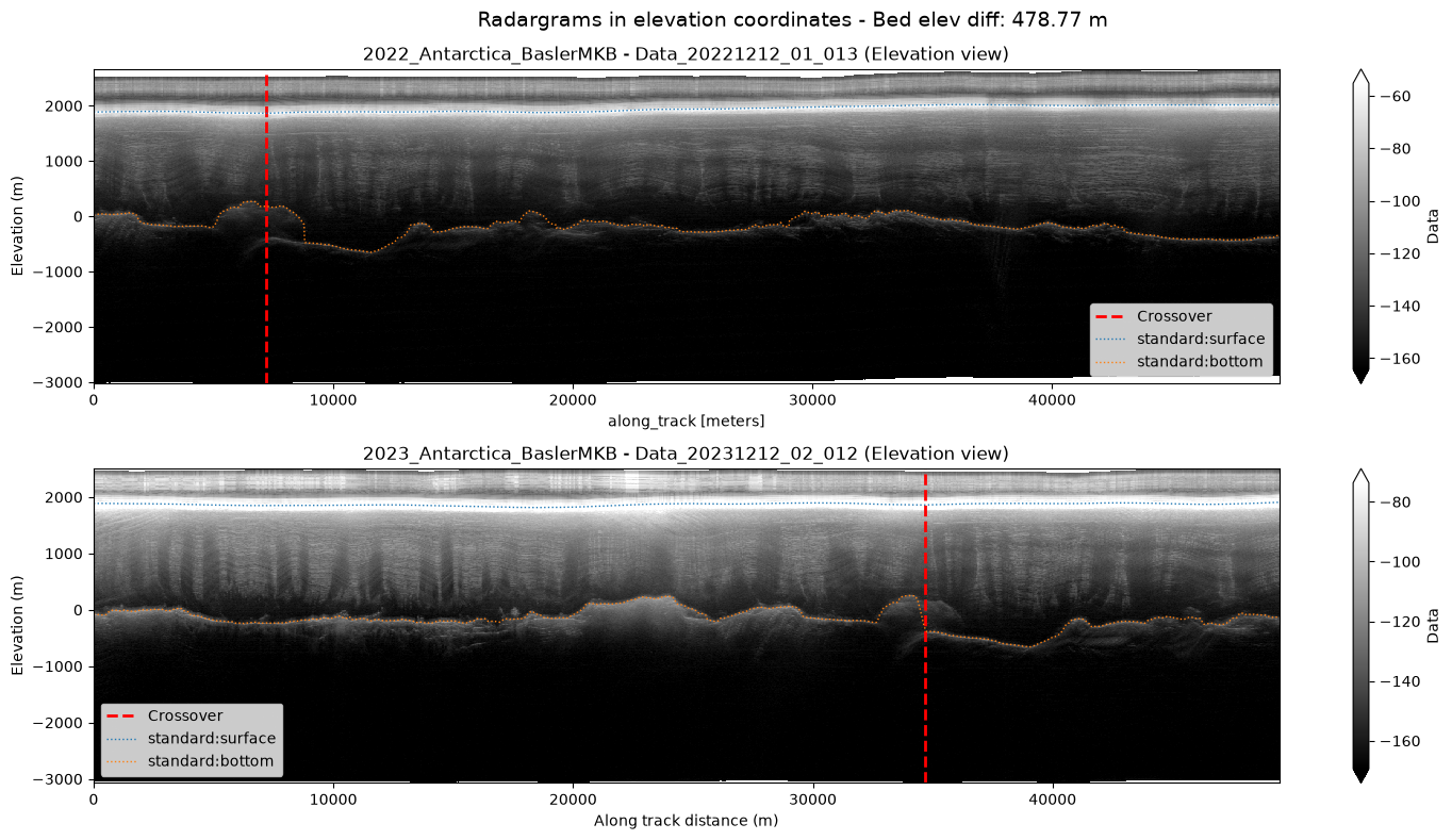

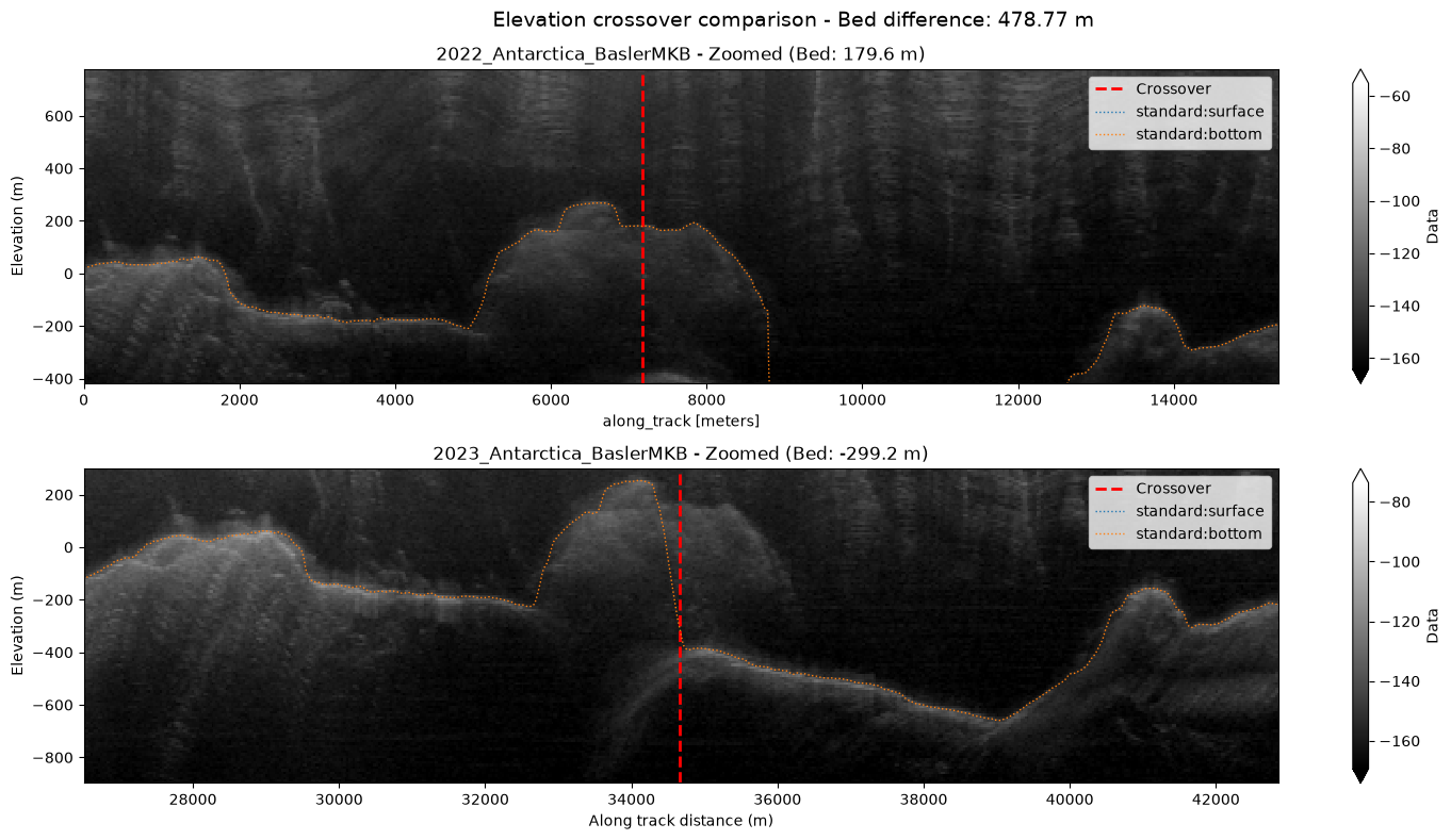
# Zoom in around the crossover point
elev_window = max(intersect['elev_diff']*2.5, 100)  # Elevation window in meters around the bed

fig, axes = plt.subplots(2, 1, figsize=(15, 8))
for k, ax in enumerate(axes):
    plot_radargram(frames[k], frame_layers[k], cross_idxs[k], ax,
                   f"{intersect[f'collection_{k+1}']} - Zoomed (Bed: {intersect[f'wgs84_{k+1}']:.1f} m)",
                   zoom=(300, elev_window))
axes[1].set_xlabel('Along track distance (m)')
plt.suptitle(f"Elevation crossover comparison - Bed difference: {intersect['elev_diff']:.2f} m", fontsize=14)
plt.tight_layout()