Open Polar Radar frames now carry per-item morton coverage (opr:mbox, four variable-resolution cells at order 18) in every STAC catalog that’s been reprocessed under issue #78. This notebook demonstrates how to combine that coverage with a single NASA CMR query for ICESat-2 ATL06 (land-ice elevation) granules to produce a GeoDataFrame of xOPR frames with a variable-length list of intersecting granules per row.
The workflow mirrors (and extends) the morton-indexed catalog pattern used in the magg library: hit CMR once, build a local index, then do all per-frame matching against the local index. We compare two matching backends against each other:
STRtree — shapely’s spatial index over projected granule polygons; exact polygon-polygon intersection per
opr:mboxcell.Morton prefix — densify each granule’s boundary, compute fine-order mortons per sample, prefix-match against each frame’s four
opr:mboxcells. Same pattern used byxopr.bedmap.morton_match.
See issue #86 for the design discussion.
import time

import fsspec
import geopandas as gpd
import matplotlib.pyplot as plt
import numpy as np
import pandas as pd

from xopr import crossovers
1. Configuration
Pick a season catalog and a temporal window for the CMR query.
Ways to specify the temporal window (resolve_temporal_window accepts any of these):
date_range=("2024-01-01", "2024-06-30")— explicit ISO dates ordatetime.dateobjects.cycle=22— an ICESat-2 repeat cycle (91 days from launch, magg-compatible).mode="exact_year"— min/max of the catalog’sopr:date. Only valid for post-2018-10-13 seasons.mode="all_years"— ICESat-2 launch (2018-10-13) to today.
The ICESat-2 ATL06 product repeats on a 91-day ground track, so for pre-launch radar seasons, choosing any full cycle still gives you useful crossovers over the same lines.
# Post-#78 catalogs with opr:mbox (current as of 2026-04). Antarctic, Bedmap-prioritized.
CATALOG_URL = (
    "https://data.source.coop/englacial/xopr/catalog/"
    "hemisphere=south/provider=cresis/collection=2016_Antarctica_DC8/stac.parquet"
)

# Pick exactly one of: DATE_RANGE, CYCLE, or TEMPORAL_MODE. The other two stay None.
DATE_RANGE = None                     # e.g. ("2024-01-01", "2024-06-30")
CYCLE = 22                            # one ICESat-2 repeat cycle (91 days); magg-compatible
TEMPORAL_MODE = None                  # "exact_year" or "all_years" — used only if the above are None

CRS = "EPSG:3031"                     # Antarctic polar stereographic

# Tunable for the prefix backend — samples per boundary edge of each granule polygon.
# ATL06 granules are thin strips so 50 is plenty.
PREFIX_N_PER_SEGMENT = 50
2. Load the xOPR STAC catalog
source.coop serves one parquet per collection; we just read it directly. The key column for this notebook is opr:mbox — gate on it and warn if missing.
with fsspec.open(CATALOG_URL) as f:
    frames = gpd.read_parquet(f)

if "opr:mbox" not in frames.columns:
    raise RuntimeError(
        "Catalog has no opr:mbox column — it predates PR #77 / issue #78. "
        "Pick a reprocessed season from https://github.com/englacial/xopr/issues/78."
    )

print(f"Loaded {len(frames)} frames from {frames['collection'].iloc[0]}")
print(f"Date range: {frames['opr:date'].min()} – {frames['opr:date'].max()}")
frames.head(3)
Loaded 1126 frames from 2016_Antarctica_DC8
Date range: 20161014 – 20161118
2b. (Optional) Subset the catalog to frames near your points
If you already have a set of (lat, lon) points of interest — e.g. rift tip locations, crossover targets, grounding-line samples — you can filter the catalog down to frames whose opr:mbox covers any of them. The check uses the same morton prefix pattern as xopr.bedmap.morton_match: each point gets an order-18 morton, and any frame whose mbox has a prefix of that morton is a hit.
Set POINTS_OF_INTEREST = None to skip this step and keep every frame.
# Example: a few Antarctic points (lat, lon). Swap in your own, or set None to skip.
POINTS_OF_INTEREST = [
    (-80.5, -78.0),   # Thwaites
    (-75.1, -105.0),  # Pine Island area
    (-70.5,  70.0),   # Amery
]

if POINTS_OF_INTEREST is not None:
    n_before = len(frames)
    frames = crossovers.subset_frames_by_points(frames, POINTS_OF_INTEREST)
    print(f"Subset by {len(POINTS_OF_INTEREST)} points: {n_before} → {len(frames)} frames")
else:
    print(f"No subset applied; working with all {len(frames)} frames")

if len(frames) == 0:
    raise RuntimeError("Subset left zero frames — widen POINTS_OF_INTEREST or set it to None.")
Subset by 3 points: 1126 → 1 frames
3. Derive the CMR bounding box
We only need a coarse spatial filter for the upstream CMR query — the per-frame matching below does the real geometric work. Union the bounding envelopes of every frame’s opr:mbox cells to get a tight footprint.
(CMR also accepts real polygon= queries with geodetic great-circle edges. We stick with a bbox here for simplicity; see issue #86 for the tradeoff.)
# Flatten every frame's 4 mbox cells into one list for the bbox computation.
all_cells = [int(c) for mbox in frames["opr:mbox"] for c in mbox]
bbox = crossovers.cmr_bbox_from_mpolygon(all_cells, step=16)
print(f"CMR bbox (lon_min, lat_min, lon_max, lat_max): {bbox}")
CMR bbox (lon_min, lat_min, lon_max, lat_max): (-105.99056603773585, -75.7091526879851, -103.5, -74.97216337509033)
4. Resolve the temporal window
start_date, end_date = crossovers.resolve_temporal_window(
    frames_gdf=frames,
    mode=TEMPORAL_MODE or "exact_year",
    cycle=CYCLE,
    date_range=DATE_RANGE,
)
print(f"Temporal window: {start_date} → {end_date}")
Temporal window: 2024-01-06 → 2024-04-06
5. One CMR query, many matches
This is the only network call to NASA CMR in the whole notebook. Everything downstream runs locally. For all_years over Antarctica, expect a few thousand ATL06 granules.
t0 = time.perf_counter()
granules = crossovers.query_cmr_granules(
    start_date=start_date,
    end_date=end_date,
    short_name="ATL06",
    version="007",
    provider="NSIDC_CPRD",
    bbox=bbox,
)
t_cmr = time.perf_counter() - t0
print(f"CMR returned {len(granules)} granules in {t_cmr:.1f}s")
CMR returned 24 granules in 0.4s
6. Match frames to granules — two backends
6a. STRtree backend
Reproject granule polygons into EPSG:3031 and build a shapely STRtree. For each frame, materialize 4 mbox cell polygons via mortie.tools.mort2polygon, reproject them, query the tree with predicate="intersects", and union the hits.
This is exact polygon-polygon intersection — the mbox cells are real polygons with great-circle/rotated shapes, not axis-aligned boxes, so we don’t collapse them to extents.
t0 = time.perf_counter()
tree, st_records = crossovers.build_granule_strtree(granules, crs=CRS)
t_build_st = time.perf_counter() - t0

t0 = time.perf_counter()
strtree_result = crossovers.match_frames_to_granules(
    frames, tree, st_records, crs=CRS, step=32,
)
t_match_st = time.perf_counter() - t0

print(f"Built STRtree over {len(st_records)} granule polygons in {t_build_st:.2f}s")
print(f"Matched {len(frames)} frames in {t_match_st:.2f}s")
strtree_result[["id", "opr:date", "opr:frame", "n_granules"]].head()
Built STRtree over 24 granule polygons in 0.00s
Matched 1 frames in 0.00s
strtree_resultstrtree_result['atl06_granules'].iloc[0][{'granule_id': 'ATL06_20240327105514_01342310_007_01.h5',
's3_url': 's3://nsidc-cumulus-prod-protected/ATLAS/ATL06/007/2024/03/27/ATL06_20240327105514_01342310_007_01.h5',
'https_url': 'https://data.nsidc.earthdatacloud.nasa.gov/nsidc-cumulus-prod-protected/ATLAS/ATL06/007/2024/03/27/ATL06_20240327105514_01342310_007_01.h5'},
{'granule_id': 'ATL06_20240125135154_05762210_007_01.h5',
's3_url': 's3://nsidc-cumulus-prod-protected/ATLAS/ATL06/007/2024/01/25/ATL06_20240125135154_05762210_007_01.h5',
'https_url': 'https://data.nsidc.earthdatacloud.nasa.gov/nsidc-cumulus-prod-protected/ATLAS/ATL06/007/2024/01/25/ATL06_20240125135154_05762210_007_01.h5'},
{'granule_id': 'ATL06_20240323110341_00732310_007_01.h5',
's3_url': 's3://nsidc-cumulus-prod-protected/ATLAS/ATL06/007/2024/03/23/ATL06_20240323110341_00732310_007_01.h5',
'https_url': 'https://data.nsidc.earthdatacloud.nasa.gov/nsidc-cumulus-prod-protected/ATLAS/ATL06/007/2024/03/23/ATL06_20240323110341_00732310_007_01.h5'},
{'granule_id': 'ATL06_20240219014935_09502212_007_01.h5',
's3_url': 's3://nsidc-cumulus-prod-protected/ATLAS/ATL06/007/2024/02/19/ATL06_20240219014935_09502212_007_01.h5',
'https_url': 'https://data.nsidc.earthdatacloud.nasa.gov/nsidc-cumulus-prod-protected/ATLAS/ATL06/007/2024/02/19/ATL06_20240219014935_09502212_007_01.h5'},
{'granule_id': 'ATL06_20240215015753_08892212_007_01.h5',
's3_url': 's3://nsidc-cumulus-prod-protected/ATLAS/ATL06/007/2024/02/15/ATL06_20240215015753_08892212_007_01.h5',
'https_url': 'https://data.nsidc.earthdatacloud.nasa.gov/nsidc-cumulus-prod-protected/ATLAS/ATL06/007/2024/02/15/ATL06_20240215015753_08892212_007_01.h5'},
{'granule_id': 'ATL06_20240117032156_04472212_007_01.h5',
's3_url': 's3://nsidc-cumulus-prod-protected/ATLAS/ATL06/007/2024/01/17/ATL06_20240117032156_04472212_007_01.h5',
'https_url': 'https://data.nsidc.earthdatacloud.nasa.gov/nsidc-cumulus-prod-protected/ATLAS/ATL06/007/2024/01/17/ATL06_20240117032156_04472212_007_01.h5'},
{'granule_id': 'ATL06_20240319002527_00052312_007_01.h5',
's3_url': 's3://nsidc-cumulus-prod-protected/ATLAS/ATL06/007/2024/03/19/ATL06_20240319002527_00052312_007_01.h5',
'https_url': 'https://data.nsidc.earthdatacloud.nasa.gov/nsidc-cumulus-prod-protected/ATLAS/ATL06/007/2024/03/19/ATL06_20240319002527_00052312_007_01.h5'},
{'granule_id': 'ATL06_20240121140015_05152210_007_01.h5',
's3_url': 's3://nsidc-cumulus-prod-protected/ATLAS/ATL06/007/2024/01/21/ATL06_20240121140015_05152210_007_01.h5',
'https_url': 'https://data.nsidc.earthdatacloud.nasa.gov/nsidc-cumulus-prod-protected/ATLAS/ATL06/007/2024/01/21/ATL06_20240121140015_05152210_007_01.h5'},
{'granule_id': 'ATL06_20240219123613_09572210_007_01.h5',
's3_url': 's3://nsidc-cumulus-prod-protected/ATLAS/ATL06/007/2024/02/19/ATL06_20240219123613_09572210_007_01.h5',
'https_url': 'https://data.nsidc.earthdatacloud.nasa.gov/nsidc-cumulus-prod-protected/ATLAS/ATL06/007/2024/02/19/ATL06_20240219123613_09572210_007_01.h5'},
{'granule_id': 'ATL06_20240117140833_04542210_007_01.h5',
's3_url': 's3://nsidc-cumulus-prod-protected/ATLAS/ATL06/007/2024/01/17/ATL06_20240117140833_04542210_007_01.h5',
'https_url': 'https://data.nsidc.earthdatacloud.nasa.gov/nsidc-cumulus-prod-protected/ATLAS/ATL06/007/2024/01/17/ATL06_20240117140833_04542210_007_01.h5'},
{'granule_id': 'ATL06_20240215124430_08962210_007_01.h5',
's3_url': 's3://nsidc-cumulus-prod-protected/ATLAS/ATL06/007/2024/02/15/ATL06_20240215124430_08962210_007_01.h5',
'https_url': 'https://data.nsidc.earthdatacloud.nasa.gov/nsidc-cumulus-prod-protected/ATLAS/ATL06/007/2024/02/15/ATL06_20240215124430_08962210_007_01.h5'},
{'granule_id': 'ATL06_20240315112020_13382210_007_01.h5',
's3_url': 's3://nsidc-cumulus-prod-protected/ATLAS/ATL06/007/2024/03/15/ATL06_20240315112020_13382210_007_01.h5',
'https_url': 'https://data.nsidc.earthdatacloud.nasa.gov/nsidc-cumulus-prod-protected/ATLAS/ATL06/007/2024/03/15/ATL06_20240315112020_13382210_007_01.h5'},
{'granule_id': 'ATL06_20240315003341_13312212_007_01.h5',
's3_url': 's3://nsidc-cumulus-prod-protected/ATLAS/ATL06/007/2024/03/15/ATL06_20240315003341_13312212_007_01.h5',
'https_url': 'https://data.nsidc.earthdatacloud.nasa.gov/nsidc-cumulus-prod-protected/ATLAS/ATL06/007/2024/03/15/ATL06_20240315003341_13312212_007_01.h5'},
{'granule_id': 'ATL06_20240319111205_00122310_007_01.h5',
's3_url': 's3://nsidc-cumulus-prod-protected/ATLAS/ATL06/007/2024/03/19/ATL06_20240319111205_00122310_007_01.h5',
'https_url': 'https://data.nsidc.earthdatacloud.nasa.gov/nsidc-cumulus-prod-protected/ATLAS/ATL06/007/2024/03/19/ATL06_20240319111205_00122310_007_01.h5'},
{'granule_id': 'ATL06_20240113033022_03862212_007_01.h5',
's3_url': 's3://nsidc-cumulus-prod-protected/ATLAS/ATL06/007/2024/01/13/ATL06_20240113033022_03862212_007_01.h5',
'https_url': 'https://data.nsidc.earthdatacloud.nasa.gov/nsidc-cumulus-prod-protected/ATLAS/ATL06/007/2024/01/13/ATL06_20240113033022_03862212_007_01.h5'},
{'granule_id': 'ATL06_20240211020615_08282212_007_01.h5',
's3_url': 's3://nsidc-cumulus-prod-protected/ATLAS/ATL06/007/2024/02/11/ATL06_20240211020615_08282212_007_01.h5',
'https_url': 'https://data.nsidc.earthdatacloud.nasa.gov/nsidc-cumulus-prod-protected/ATLAS/ATL06/007/2024/02/11/ATL06_20240211020615_08282212_007_01.h5'},
{'granule_id': 'ATL06_20240311004211_12702212_007_01.h5',
's3_url': 's3://nsidc-cumulus-prod-protected/ATLAS/ATL06/007/2024/03/11/ATL06_20240311004211_12702212_007_01.h5',
'https_url': 'https://data.nsidc.earthdatacloud.nasa.gov/nsidc-cumulus-prod-protected/ATLAS/ATL06/007/2024/03/11/ATL06_20240311004211_12702212_007_01.h5'},
{'granule_id': 'ATL06_20240109033842_03252212_007_01.h5',
's3_url': 's3://nsidc-cumulus-prod-protected/ATLAS/ATL06/007/2024/01/09/ATL06_20240109033842_03252212_007_01.h5',
'https_url': 'https://data.nsidc.earthdatacloud.nasa.gov/nsidc-cumulus-prod-protected/ATLAS/ATL06/007/2024/01/09/ATL06_20240109033842_03252212_007_01.h5'},
{'granule_id': 'ATL06_20240207021440_07672212_007_01.h5',
's3_url': 's3://nsidc-cumulus-prod-protected/ATLAS/ATL06/007/2024/02/07/ATL06_20240207021440_07672212_007_01.h5',
'https_url': 'https://data.nsidc.earthdatacloud.nasa.gov/nsidc-cumulus-prod-protected/ATLAS/ATL06/007/2024/02/07/ATL06_20240207021440_07672212_007_01.h5'},
{'granule_id': 'ATL06_20240227121929_10792210_007_01.h5',
's3_url': 's3://nsidc-cumulus-prod-protected/ATLAS/ATL06/007/2024/02/27/ATL06_20240227121929_10792210_007_01.h5',
'https_url': 'https://data.nsidc.earthdatacloud.nasa.gov/nsidc-cumulus-prod-protected/ATLAS/ATL06/007/2024/02/27/ATL06_20240227121929_10792210_007_01.h5'},
{'granule_id': 'ATL06_20240121031337_05082212_007_01.h5',
's3_url': 's3://nsidc-cumulus-prod-protected/ATLAS/ATL06/007/2024/01/21/ATL06_20240121031337_05082212_007_01.h5',
'https_url': 'https://data.nsidc.earthdatacloud.nasa.gov/nsidc-cumulus-prod-protected/ATLAS/ATL06/007/2024/01/21/ATL06_20240121031337_05082212_007_01.h5'}]6b. Morton prefix backend
For each granule, densify the CMR-reported boundary and compute a full-order (order 18) morton for every sample. For each frame mbox cell (a variable-length prefix string), any granule whose sample morton starts with that prefix overlaps the cell. Same string-prefix pattern used by xopr.bedmap.morton_match — it generalizes from points to polygons by sampling.
t0 = time.perf_counter()
pf_records = crossovers.build_granule_prefix_index(
    granules, n_per_segment=PREFIX_N_PER_SEGMENT,
)
t_build_pf = time.perf_counter() - t0

t0 = time.perf_counter()
prefix_result = crossovers.match_frames_to_granules_prefix(frames, pf_records)
t_match_pf = time.perf_counter() - t0

print(f"Built prefix index over {len(pf_records)} granules in {t_build_pf:.2f}s")
print(f"Matched {len(frames)} frames in {t_match_pf:.2f}s")
prefix_result[["id", "opr:date", "opr:frame", "n_granules"]].head()
Built prefix index over 24 granules in 0.02s
Matched 1 frames in 0.02s
timing = pd.DataFrame(
    {
        "stage": ["index build", "frame matching", "total local"],
        "STRtree (s)": [t_build_st, t_match_st, t_build_st + t_match_st],
        "prefix (s)": [t_build_pf, t_match_pf, t_build_pf + t_match_pf],
    }
)
timing["prefix / STRtree"] = timing["prefix (s)"] / timing["STRtree (s)"]
timing.style.format("{:.3f}", subset=["STRtree (s)", "prefix (s)", "prefix / STRtree"])7b. Per-frame hit agreement
We treat the STRtree result as ground truth (exact polygon intersection) and ask: how often does the prefix backend miss a true hit, and how often does it over-report?
def _ids(row):
    return {g["granule_id"] for g in row}

st_sets = strtree_result["atl06_granules"].apply(_ids)
pf_sets = prefix_result["atl06_granules"].apply(_ids)

missed_by_prefix = [len(st - pf) for st, pf in zip(st_sets, pf_sets)]
extra_from_prefix = [len(pf - st) for st, pf in zip(st_sets, pf_sets)]

summary = pd.DataFrame(
    {
        "STRtree n_granules": strtree_result["n_granules"],
        "prefix n_granules": prefix_result["n_granules"],
        "missed by prefix": missed_by_prefix,
        "extra from prefix": extra_from_prefix,
    }
)
print(f"Frames with any disagreement: {(summary['missed by prefix'] + summary['extra from prefix'] > 0).sum()}/{len(summary)}")
print(f"Mean missed by prefix: {np.mean(missed_by_prefix):.2f}")
print(f"Mean extra from prefix: {np.mean(extra_from_prefix):.2f}")
summary.describe()
Frames with any disagreement: 1/1
Mean missed by prefix: 0.00
Mean extra from prefix: 1.00
What to expect:
STRtree is exact — every hit corresponds to a real polygon-polygon intersection.
Prefix can miss — if a frame’s mbox cell lies entirely inside a granule with none of the densified boundary samples landing in the cell. In practice rare for thin ATL06 strips at default
n_per_segment=50; raise the knob if your missed count is nonzero.Prefix can over-report — an
opr:mboxcell overapproximates the frame’s true geometry (mortie rounds up to cell boundaries), so a granule touching the cell but not the line string still counts as a hit. This is the same overapproximation inherent toopr:mbox, not specific to the prefix backend.
For large catalogs where granules outnumber frames, STRtree is usually faster to match because polygon intersection short-circuits in log-time via the spatial index; prefix matching is O(frames × granules × samples × 4).
8. Final result: frame → granule table
We carry the STRtree result forward (exact), but the prefix result has the same schema and is drop-in compatible. Each row is an xOPR frame; atl06_granules is a variable-length list of dicts (granule_id, s3_url, https_url) so downstream code can pick the URL flavor that suits its auth context.
result = strtree_result
print(f"{len(result)} frames, {result['n_granules'].sum()} total frame↔granule edges")
print(f"Frames with ≥1 granule: {(result['n_granules'] > 0).sum()} ({100*(result['n_granules'] > 0).mean():.1f}%)")
print(f"Median granules per frame: {int(result['n_granules'].median())}")
result[["id", "opr:segment", "opr:date", "opr:frame", "geometry", "atl06_granules", "n_granules"]].head()
1 frames, 21 total frame↔granule edges
Frames with ≥1 granule: 1 (100.0%)
Median granules per frame: 21
# Show the granules for one frame with hits
hit = result[result["n_granules"] > 0].iloc[0]
print(f"Frame {hit['id']} matches {hit['n_granules']} ATL06 granules.")
print("First three:")
for g in hit["atl06_granules"][:3]:
    print(f"  {g['granule_id']}")
    print(f"    s3:    {g['s3_url']}")
    print(f"    https: {g['https_url']}")
Frame Data_20161103_06_010 matches 21 ATL06 granules.
First three:
ATL06_20240327105514_01342310_007_01.h5
s3: s3://nsidc-cumulus-prod-protected/ATLAS/ATL06/007/2024/03/27/ATL06_20240327105514_01342310_007_01.h5
https: https://data.nsidc.earthdatacloud.nasa.gov/nsidc-cumulus-prod-protected/ATLAS/ATL06/007/2024/03/27/ATL06_20240327105514_01342310_007_01.h5
ATL06_20240125135154_05762210_007_01.h5
s3: s3://nsidc-cumulus-prod-protected/ATLAS/ATL06/007/2024/01/25/ATL06_20240125135154_05762210_007_01.h5
https: https://data.nsidc.earthdatacloud.nasa.gov/nsidc-cumulus-prod-protected/ATLAS/ATL06/007/2024/01/25/ATL06_20240125135154_05762210_007_01.h5
ATL06_20240323110341_00732310_007_01.h5
s3: s3://nsidc-cumulus-prod-protected/ATLAS/ATL06/007/2024/03/23/ATL06_20240323110341_00732310_007_01.h5
https: https://data.nsidc.earthdatacloud.nasa.gov/nsidc-cumulus-prod-protected/ATLAS/ATL06/007/2024/03/23/ATL06_20240323110341_00732310_007_01.h5
9. Quick map: frames coloured by granule hit count
A matplotlib scatter in EPSG:3031 to sanity-check the spatial distribution of hits.
result_3031 = result.to_crs(CRS)
fig, ax = plt.subplots(1, 1, figsize=(9, 9))
result_3031.plot(
    column="n_granules",
    cmap="viridis",
    linewidth=0.6,
    legend=True,
    ax=ax,
)
ax.set_title(f"{frames['collection'].iloc[0]} — ATL06 hits per frame")
ax.set_xlabel("x (m, EPSG:3031)")
ax.set_ylabel("y (m, EPSG:3031)")
ax.set_aspect("equal")
plt.tight_layout()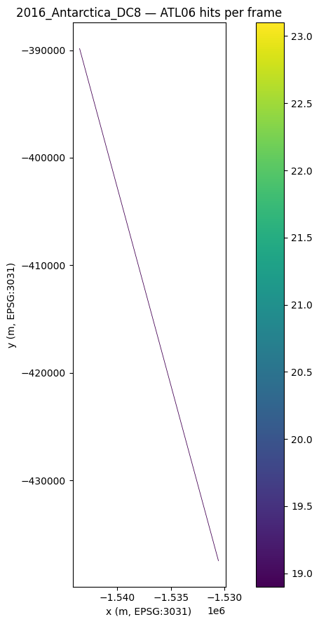
Follow-ups
Planned (see issue #86):
Read-along demo — pick a frame with hits, open a matched ATL06 granule via h5coro or icepyx, clip to a buffer around the frame LineString, and co-plot ATL06 surface elevations against the frame’s radar echogram / picked surface layer.
Reverse direction — given one ATL06 ground track, find every xOPR frame across all seasons that crosses it.
Persistent local catalog — mirror magg’s on-disk JSON catalog so repeated notebook runs don’t hit CMR.
Unified prefix core — share one prefix-matching implementation between
xopr.bedmap.morton_matchandxopr.crossoversonce both workflows are stable.