Layer picks in OPR data (such as the surface and bed layers) should be pretty good, but they’re not always perfect. Sometimes the pick is offset from the true reflection peak by a few samples, and occasionally it’s just wrong. If your work relies on having exactly the right surface or bed point, you may want to consider locally repicking.
“Repicking” refers to refining these layer picks by examining the radar data in a local window around each existing pick and selecting a better value. This notebook demonstrates two approaches:
Local maximum: Simply take the strongest return within a window around the existing pick.
scipy.signal.find_peaks: Use peak detection with custom parameters for more control over the selection criteria.
import numpy as np
import xarray as xr
import matplotlib.pyplot as plt
from scipy.signal import find_peaks

import xopr

import holoviews as hv
import hvplot.xarray
hvplot.extension('bokeh')opr = xopr.OPRConnection(cache_dir="radar_cache")Load a flight line and its layer picks
We’ll start by loading a flight segment and its existing layer picks.
collection = "2008_Antarctica_BaslerJKB"
segment = "20090126_02"

stac_items = opr.query_frames(collections=collection, segment_paths=[segment])
frames = opr.load_frames(stac_items)
flight_line = xopr.merge_frames(frames)
/home/runner/work/xopr/xopr/src/xopr/opr_access.py:481: UserWarning: Warning: Unexpected result from ops_api: ERROR: SEGMENT DOES NOT EXIST.
warnings.warn(f"Warning: Unexpected result from ops_api: {result['data']}", UserWarning)
layers = opr.get_layers(flight_line)
print("Available layers:", list(layers.keys()))

# Prepare data for repicking: linear power with dims (twtt, slow_time)
linear_data = np.abs(flight_line['Data']).transpose('twtt', 'slow_time')

# Prepare dB version for display only
radargram_db = 10 * np.log10(linear_data)
radargram_db.name = 'Power (dB)'
Available layers: ['standard:surface', 'standard:bottom']
Defining repick functions
The idea behind repicking is simple: for each trace, look at the radar data in a small window around the existing pick and choose a better twtt value. The choice of how to pick within that window is where the two approaches differ.
We define two small functions that operate on a single trace. Both have the same signature — they take a 1D trace array, a scalar pick value, and the twtt coordinate array, and return a scalar twtt value. This means either one can be plugged into the same repick() driver via xr.apply_ufunc.
def local_max(trace, pick_twtt_val, twtt_vals, window_size):
    """Take the maximum amplitude within ±window_size samples of the pick."""
    if np.isnan(pick_twtt_val):
        return np.nan
    dt = twtt_vals[1] - twtt_vals[0]
    idx = int(np.round((pick_twtt_val - twtt_vals[0]) / dt))
    if idx < 0 or idx >= len(twtt_vals):
        return np.nan
    lo, hi = max(0, idx - window_size), min(len(twtt_vals), idx + window_size + 1)
    window = trace[lo:hi]
    if np.all(np.isnan(window)):
        return pick_twtt_val
    return twtt_vals[lo + np.nanargmax(window)]


def find_peaks_local(trace, pick_twtt_val, twtt_vals, window_size, rel_prominence=0.1, **kwargs):
    """Run find_peaks in a window around the pick; return the closest prominent peak."""
    if np.isnan(pick_twtt_val):
        return np.nan
    dt = twtt_vals[1] - twtt_vals[0]
    idx = int(np.round((pick_twtt_val - twtt_vals[0]) / dt))
    if idx < 0 or idx >= len(twtt_vals):
        return np.nan
    lo, hi = max(0, idx - window_size), min(len(twtt_vals), idx + window_size + 1)
    window = np.nan_to_num(trace[lo:hi], nan=0.0)
    peaks, _ = find_peaks(window, prominence=rel_prominence * np.max(window), **kwargs)
    if len(peaks) == 0:
        return pick_twtt_val
    closest = peaks[np.argmin(np.abs(peaks - (idx - lo)))]
    return twtt_vals[lo + closest]
The driver function repick() uses xr.apply_ufunc to apply either of the above functions across all traces. The input_core_dims=[['twtt'], []] tells xarray to pass each trace as a 1D array and each pick as a scalar. You swap the repicking strategy simply by passing a different func.
def repick(data, pick_twtt, func, window_size=50, **kwargs):
    """
    Repick a layer by applying func to each trace.

    Parameters
    ----------
    data : xr.DataArray
        Radar data with a 'twtt' dimension (linear power, not dB).
    pick_twtt : xr.DataArray
        Existing layer picks as twtt values, indexed by slow_time.
    func : callable
        Per-trace repick function with signature (trace, pick_twtt_val, twtt_vals, window_size, **kwargs) -> float.
        Use `local_max` or `find_peaks_local`.
    window_size : int
        Half-width of the search window in number of samples.
    **kwargs
        Extra keyword arguments forwarded to func (e.g. rel_prominence, distance).
    """
    pick_aligned = pick_twtt.interp(slow_time=data['slow_time'], method='nearest')
    return xr.apply_ufunc(
        func, data, pick_aligned,
        input_core_dims=[['twtt'], []],
        output_core_dims=[[]],
        vectorize=True,
        kwargs=dict(twtt_vals=data['twtt'].values, window_size=window_size, **kwargs),
    )
Running the repick
Both functions work on the linear-power data (not the dB version). We call repick() with each function — the only thing that changes is which func we pass and any extra keyword arguments it needs.
find_peaks_local takes a rel_prominence parameter that sets the prominence threshold as a fraction of each window’s maximum. This is important because the surface return is orders of magnitude stronger than the bed — an absolute prominence threshold would either accept every noise peak near the surface or reject every real peak near the bed.
# Method 1: local maximum — just takes the strongest return in the window
bed_repicked_max = repick(linear_data, layers['standard:bottom']['twtt'], local_max, window_size=50)
surface_repicked_max = repick(linear_data, layers['standard:surface']['twtt'], local_max, window_size=30)

# Method 2: find_peaks — uses prominence to pick the best real peak
bed_repicked_peaks = repick(linear_data, layers['standard:bottom']['twtt'], find_peaks_local,
                            window_size=50, rel_prominence=0.1, distance=5)
surface_repicked_peaks = repick(linear_data, layers['standard:surface']['twtt'], find_peaks_local,
                                window_size=30, rel_prominence=0.1)
Single-trace diagnostic
Before looking at the full flight line, it’s helpful to examine a single trace to understand what the repicking is doing. Here we plot the radar amplitude in a window around the bed pick and mark the peaks that find_peaks identifies:
# Look at a single trace near the middle of the flight
trace_idx = len(linear_data['slow_time']) // 2
trace = linear_data.isel(slow_time=trace_idx).values

bed_pick_aligned = layers['standard:bottom']['twtt'].interp(slow_time=linear_data['slow_time'], method='nearest')
bed_twtt = float(bed_pick_aligned.isel(slow_time=trace_idx).values)
twtt_vals = linear_data['twtt'].values
dt = twtt_vals[1] - twtt_vals[0]

bed_idx = int(np.round((bed_twtt - twtt_vals[0]) / dt))
window_size = 50
lo, hi = max(0, bed_idx - window_size), min(len(twtt_vals), bed_idx + window_size + 1)

window = np.nan_to_num(trace[lo:hi], nan=0.0)
peaks_all, _ = find_peaks(window)
peaks_prominent, _ = find_peaks(window, prominence=0.1 * np.max(window))

fig, ax = plt.subplots(figsize=(10, 4))
ax.plot(twtt_vals[lo:hi] * 1e6, trace[lo:hi], 'k-', linewidth=0.8)
ax.axvline(bed_twtt * 1e6, color='tab:blue', linestyle=':', label='Original pick')
ax.plot(twtt_vals[lo + peaks_all] * 1e6, trace[lo + peaks_all], 'v', color='tab:gray', markersize=6, label=f'All peaks ({len(peaks_all)})')
ax.plot(twtt_vals[lo + peaks_prominent] * 1e6, trace[lo + peaks_prominent], '^', color='tab:red', markersize=8, label=f'Prominent peaks ({len(peaks_prominent)})')
ax.set_xlabel('TWTT (μs)')
ax.set_ylabel('Amplitude')
ax.set_title('Single trace: peaks around the bed pick')
ax.legend()
plt.show()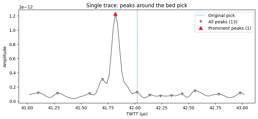
Comparing the results
Let’s compare the original bed picks with the two repicked versions. First a full flight line view, then a zoom:
fig, ax = plt.subplots(figsize=(15, 4))
radargram_db.plot.pcolormesh(x='slow_time', cmap='gray', ax=ax)
ax.invert_yaxis()

layers['standard:bottom']['twtt'].plot(ax=ax, x='slow_time', linewidth=0.5, linestyle=':', color='tab:blue', label='Original')
bed_repicked_max.plot(ax=ax, linewidth=0.5, color='tab:cyan', label='Local max')
bed_repicked_peaks.plot(ax=ax, linewidth=0.5, color='tab:red', label='find_peaks')
ax.legend(loc='upper right')
ax.set_title("Bed picks: original vs repicked")
plt.show()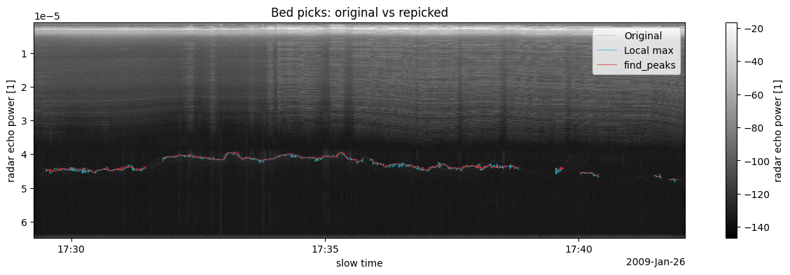
# Zoom in on ~200 traces near the middle, tight twtt range around the bed
n_traces = len(radargram_db['slow_time'])
zmid = n_traces // 2
zlo, zhi = zmid - 100, zmid + 100

zoom_st = radargram_db['slow_time'].values[zlo:zhi]
st_lo, st_hi = zoom_st[0], zoom_st[-1]

bed_aligned = layers['standard:bottom']['twtt'].interp(slow_time=radargram_db['slow_time'], method='nearest')
bed_slice = bed_aligned.values[zlo:zhi]
bed_valid = bed_slice[np.isfinite(bed_slice)]
twtt_pad = 3e-6
twtt_lo, twtt_hi = bed_valid.min() - twtt_pad, bed_valid.max() + twtt_pad

fig, axes = plt.subplots(1, 3, figsize=(16, 5), sharey=True)

for i, (ax, title, repicked) in enumerate(zip(
    axes,
    ['Original only', 'Local max', 'find_peaks'],
    [None, bed_repicked_max, bed_repicked_peaks],
)):
    im = radargram_db.plot.pcolormesh(x='slow_time', cmap='gray', ax=ax, add_colorbar=False)
    ax.invert_yaxis()
    layers['standard:bottom']['twtt'].plot(
        ax=ax, x='slow_time', linewidth=1.5, linestyle='--', color='tab:blue', label='Original'
    )
    if repicked is not None:
        repicked.plot(ax=ax, linewidth=1.5, color='tab:red', marker='.', markersize=3, label=title)
    ax.set_xlim(st_lo, st_hi)
    ax.set_ylim(twtt_hi, twtt_lo)
    ax.set_title(title)
    ax.legend(loc='lower right', fontsize=8)
    if ax != axes[0]:
        ax.set_ylabel('')

fig.colorbar(im, ax=axes, label='Power (dB)', shrink=0.8)
plt.show()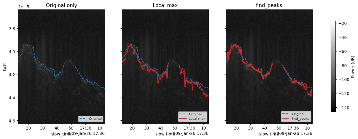
Quantifying the difference
It can be helpful to see how much the repicked values differ from the originals. Large differences might indicate either a successful correction or a bad pick that needs manual review.
# Align original picks to the same slow_time grid as the repicked values
bed_original = layers['standard:bottom']['twtt'].interp(slow_time=linear_data['slow_time'], method='nearest')

bed_diff_max = (bed_repicked_max - bed_original) * 1e6
bed_diff_peaks = (bed_repicked_peaks - bed_original) * 1e6

fig, axes = plt.subplots(1, 2, figsize=(14, 3), sharey=True)

axes[0].hist(bed_diff_max.values[np.isfinite(bed_diff_max.values)], bins=100, color='tab:cyan')
axes[0].set_xlabel('ΔTWTT (μs)')
axes[0].set_ylabel('Count')
axes[0].set_title('Bed: local max − original')

axes[1].hist(bed_diff_peaks.values[np.isfinite(bed_diff_peaks.values)], bins=100, color='tab:red')
axes[1].set_xlabel('ΔTWTT (μs)')
axes[1].set_title('Bed: find_peaks − original')

plt.tight_layout()
plt.show()

for name, diff in [("Local max", bed_diff_max), ("find_peaks", bed_diff_peaks)]:
    valid = diff.values[np.isfinite(diff.values)]
    if len(valid) == 0:
        print(f"{name}: no valid comparisons")
        continue
    print(f"{name}: median shift = {np.median(valid):.4f} μs, "
          f"mean |shift| = {np.mean(np.abs(valid)):.4f} μs, "
          f"max |shift| = {np.max(np.abs(valid)):.4f} μs")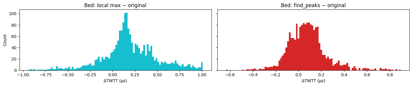
Local max: median shift = 0.1669 μs, mean |shift| = 0.2866 μs, max |shift| = 1.0087 μs
find_peaks: median shift = 0.0675 μs, mean |shift| = 0.1384 μs, max |shift| = 0.8949 μs
Interactive radargram
The plot below uses HoloViews/Bokeh — use the scroll wheel to zoom and drag to pan.
Original picks are shown as dashed lines. Repicked versions are solid: cyan for local max, red for find_peaks.
# Subsample for interactive plotting (full resolution is too large without datashader)
step = max(1, len(radargram_db['slow_time']) // 500)
radargram_sub = radargram_db.isel(slow_time=slice(None, None, step))

radargram_hv = radargram_sub.hvplot.quadmesh(
    x='slow_time', y='twtt', cmap='gray',
    width=900, height=500, colorbar=True, clabel='Power (dB)',
).opts(invert_yaxis=True)

def _curve(da, label, color, dash='solid'):
    """Helper to build an hv.Curve from an xr.DataArray or layer dataset."""
    return hv.Curve(
        (da['slow_time'].values, da.values), 'slow_time', 'twtt', label=label
    ).opts(color=color, line_dash=dash, line_width=1.5)

# Original picks (dashed)
surf_orig = _curve(layers['standard:surface']['twtt'], 'Surface (original)', 'blue', 'dashed')
bed_orig = _curve(layers['standard:bottom']['twtt'], 'Bed (original)', 'blue', 'dashed')

# Local max repicks (cyan solid)
surf_max = _curve(surface_repicked_max, 'Surface (local max)', 'cyan')
bed_max = _curve(bed_repicked_max, 'Bed (local max)', 'cyan')

# find_peaks repicks (red solid)
surf_fp = _curve(surface_repicked_peaks, 'Surface (find_peaks)', 'red')
bed_fp = _curve(bed_repicked_peaks, 'Bed (find_peaks)', 'red')

(radargram_hv * surf_orig * bed_orig * surf_max * bed_max * surf_fp * bed_fp).opts(
    title='Interactive comparison — zoom in to see differences',
    active_tools=['wheel_zoom'],
    legend_position='top_left',
)